Graphing a Circle
It is cumbersome to graph a function in rectangular coordinate form that has multiple points for a single $x$ value. For example, when trying to graph a circle from equation $x^2+y^2=r^2$ we may typically only get the top or bottom half of it depending on the sign chosen. $y=\pm\sqrt{1-x^2}$. In order to get the whole circle, we have to graph $y=\sqrt{1-x^2}$ and then graph $y=-\sqrt{1-x^2}$.
An alternative method is to plot the function as a vector valued function, also in this instance called a parametric function. In the section on parametric curves, I show how to derive the parametrized form, so here I just note that the whole circle is easily graphed this way.
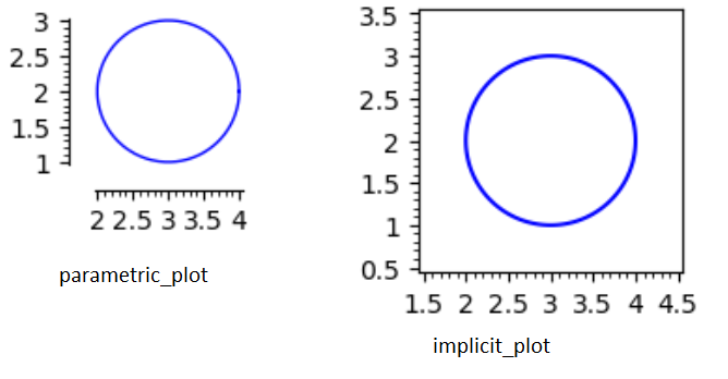
h=3; k=2;
parametric_plot(cos(x)+h,sin(x)+k],(x,0,2*pi))
The implicit plot uses different code:
f(x,y)=(x-3)^2 + (y-2)^2-1
implicit_plot(f,(1.5,4.5),(0.5,3.5))
But, they both draw the same circle.
As computer graphic software has advanced, it is now ever more common to see automatic plotting of "implicit" equations. If we look at Sagemath, which is an open source computer algebra system developed by William Stein, we find a relatively easy method for input of parametric equations, as well as an implicit plot function which avoids having to solve equations in order to view their graph.
import matplotlib.pyplot as plt
import numpy as np
t = np.linspace(0,np.pi*2,30)
fig = plt.figure()
ax = fig.add_subplot(111)
ax.set_aspect('equal')
for tval in t:
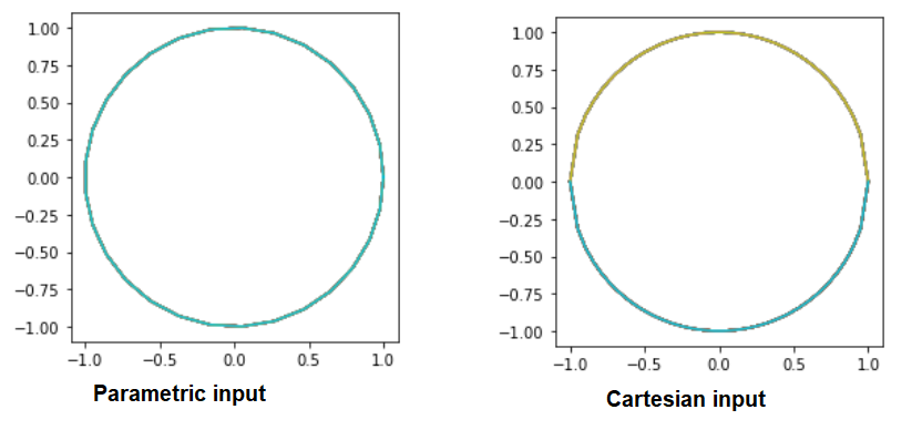
ax.plot(np.cos(t),np.sin(t))
plt.show()
The Cartesian plot is actually produced by graphing both positive and negative portions of the root. Its code is
import matplotlib.pyplot as plt
import numpy as np
x = np.linspace(-1,1,40)
fig = plt.figure()
ax = fig.add_subplot(111)
ax.set_aspect('equal')
for tval in x:
ax.plot(x,np.sqrt(1-x**2))
ax.plot(x,-np.sqrt(1-x**2))
plt.show()
But, they both draw the same circle.
Most computer languages, make it a little more involved to make graphs. Even though Sagemath is based on Python, using exclusively Python, even with the normal library imports, the graphs of something as simple as a circle require several lines of code. In addition, the python rendering has to have extra code added in to assure an equal aspect ratio.
In the higher level language, Octave, with syntax nearly the same as Matlab, a parametric circle can be plotted in only two lines.
t = 0: 0.01: 2*pi;
plot(cos(t),sin(t))
However, to graph the Cartesian equation $(x-h)^2+(y-k)^2=r^2$ requires quite a few lines of code, with a strategy similar to that used with python.
The application, Geogebra, is not really a programming language, albeit some scripting is possible. It defauts to an implict plot with input $x^{2}+y^{2}=1$ and also defaults to a parametric circle plot with input $(\cos(t),\sin(t))$.
Graphing calculators such as the TI Nspire CXII will accept parametric input, although many others only graph a function of one variable, which means no implicit plots.
If graphing is the only interest, then online applications like Wolfram alpha will readily accommodate most functions of one or two variables and will do some 3-dimensional equations as well.